Solid-state battery,
driven by Claude Code.

FastF1 → race-winner's fastest lap

The Python script connects to FastF1 3.8.1, loads the 2026 Miami GP race session, picks the winner from session.results, and pulls the fastest lap car-data via pick_drivers().pick_fastest().get_car_data(). The first run of the season triggers a cold cache fill against the F1 timing API — every run after that hits the local ~/fastf1_cache, so iteration is instant.

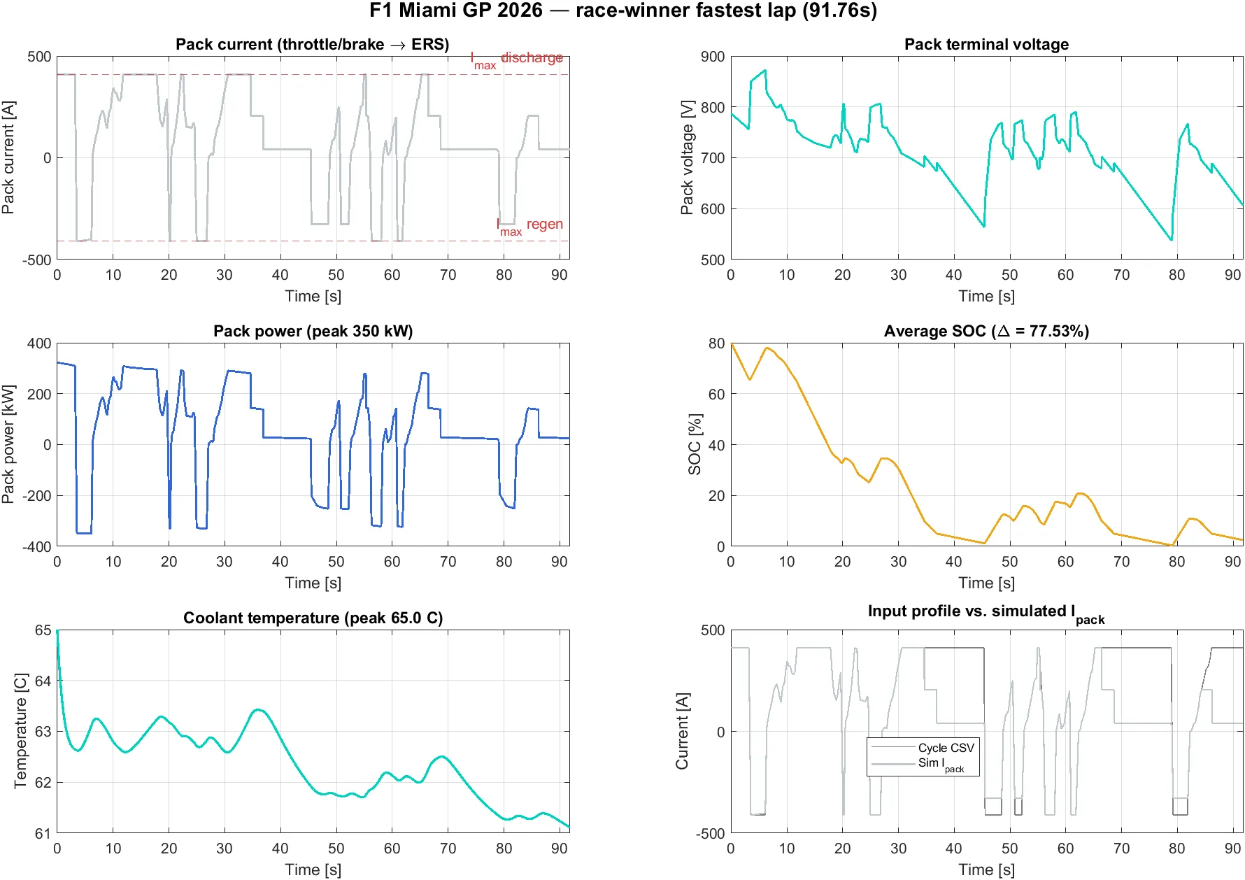
The car-data trace for the winner's fastest race lap contains 328 samples covering 91.76 s, with speed ranging 65–327 km/h, throttle on for 63.8 % of the lap and brake active 16.5 % of the lap. The fastest race lap landed at 1:31.968 on lap 34.

Throttle & brake → ERS deploy & regen

Real F1 ERS is governed by the engine map and the driver's MGU-K request, but for this study a deliberately simple, physics-defensible mapping is enough: throttle percentage drives the pack discharge current and braking events trigger regen charge, both clipped to the BMS-defined ±410 A pack limits. When brake is on, throttle contribution is zeroed defensively.

For the Miami winner's lap that produces a current trace with mean +192 A, RMS 353 A, peaks at -410 A on hard braking and +410 A on full-throttle pulls. The single-lap input profile is the file the Simulink model consumes verbatim — profile_miami_gp_2026.csv ships in the project's Test cycles/ folder alongside the other canonical bench cycles.

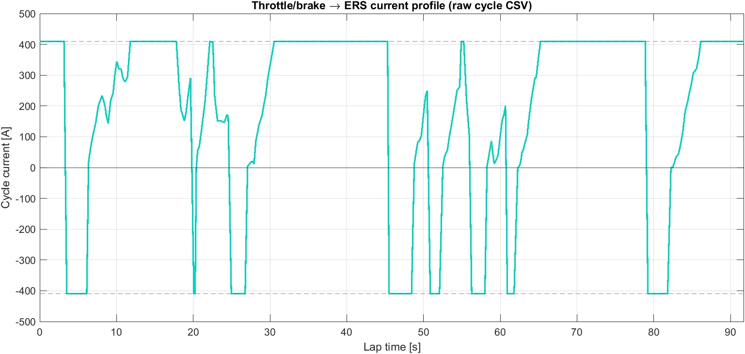
// scripts/fetch_miami_gp_2026.py — race-winner fastest lap
session = fastf1.get_session(2026, "Miami", "R")
session.load(telemetry=True, laps=True)

winner  = session.results.iloc[0]              # Race winner
fastest = session.laps.pick_drivers(winner["Abbreviation"]).pick_fastest()
car     = fastest.get_car_data().add_distance() # 328 samples · 91.76 s · 65–327 km/h

# Throttle (0..100)  →  ERS discharge current
# Brake   (bool)     →  ERS regen     current
discharge = (car["Throttle"] / 100) * I_MAX_DISCHARGE
regen     = -car["Brake"].astype(float) * I_MAX_REGEN
discharge = np.where(car["Brake"], 0.0, discharge)
current_A = np.clip(discharge + regen, -410, +410)

Electro-thermal cell — composite PEO/LLZO + NMC622

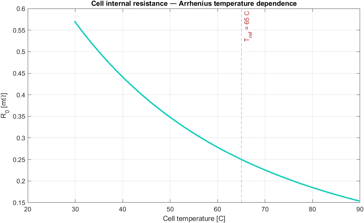
Each cell in the pack is the same MATLAB Function block — ssb_cell_model_fcn — coupled to a thermal sub-block. The internal resistance follows an Arrhenius temperature law with literature-anchored reference resistance and activation energy, the OCV is a literature lookup against state of charge, the entropy coefficient drives reversible heating, and a single RC pair captures diffusion dynamics. Heat from I²R losses and the entropy term feeds into a thermal node with cell mass, specific heat and convection to the dielectric oil.

The chemistry choice — composite PEO/LLZO solid electrolyte with single-ion copolymers, an ultra-thin membrane and a power-optimised multi-stack pouch design — is what makes the headline pack numbers possible. The composite drops the activation energy for ionic conductivity well below neat amorphous PEO, and tabless current collectors plus a LiF/LLZO interface buffer take the cell-level resistance down to a small fraction of what a conventional PEO build would deliver. None of that came from speculation — every parameter has a literature anchor.

Pack, oil-immersion cooling, governed pack

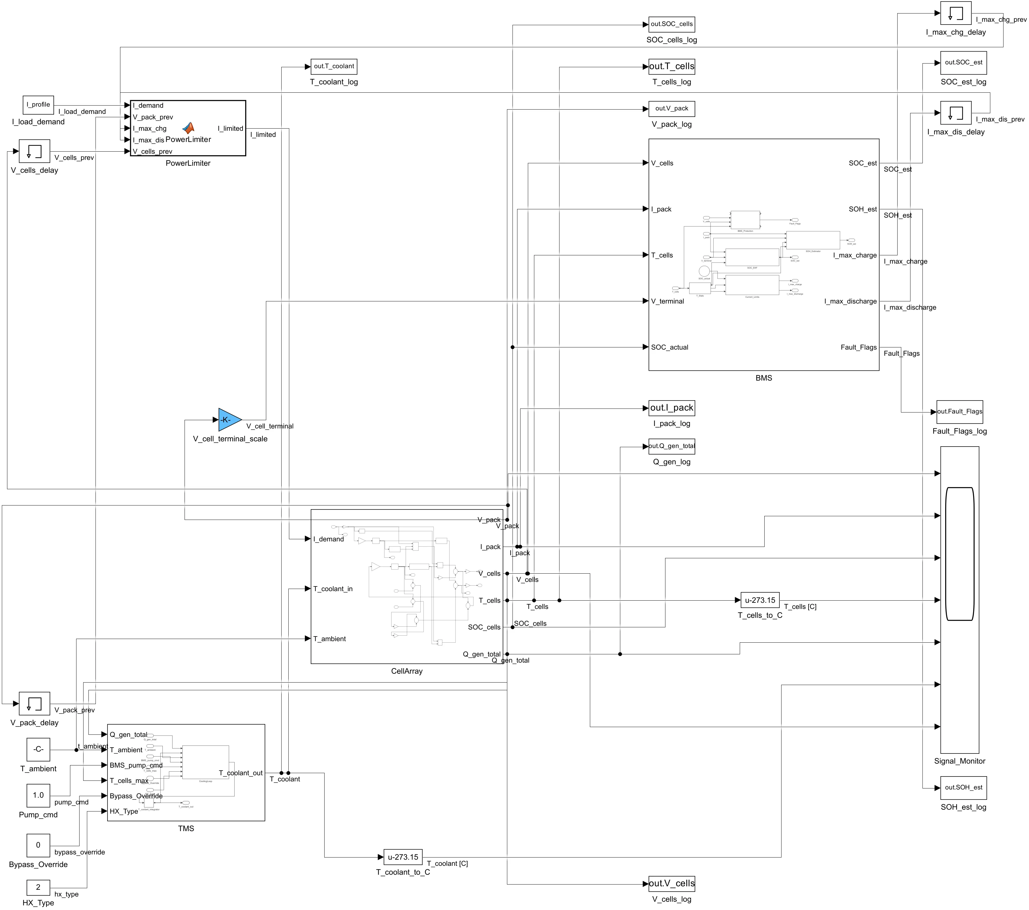
Cells are assembled in series into an 850 V / 2.17 kWh pack. Cooling is dielectric-oil immersion: each cell sees a convective heat-transfer coefficient against a lumped coolant mass, with a variable-speed pump throttled by a temperature-aware control law that keeps the pack inside the PEO operating window.

The BMS sits between the requested current and the pack. Protection thresholds are V_cell ∈ [2.50, 4.25] V and T_cell ∈ [40, 80] °C; a Derating_Logic block derates allowable charge/discharge current as the cell approaches voltage or thermal limits; an EKF estimates SOC from cell voltage + current; an Ah-counter cross-checks. A 5 kW PTC pre-heater wakes when the pack is below 55 °C and shuts off at 65 °C — necessary because PEO conductivity collapses below 60 °C.

Live MATLAB session, single MCP tool call

The MATLAB MCP server attaches to a running R2023a session — same session the engineer would use interactively — so every cd, load_system, set_param and sim happens in the same workspace, with the same paths, the same warnings, the same output. Claude Code dispatches one evaluate_matlab_code tool call that runs scripts/run_f1_miami_gp_2026.m; the script loads the master parameter file, builds I_profile in the base workspace, kills EnablePacing (golden rule — pacing forces real-time playback and would make sweeps unusable), runs the simulation, extracts logged signals, computes headline metrics, exports three PNGs through exportgraphics and saves a MAT file for the page.

Wall-time for the 91.76 s lap is 4.69 s — about 20× real-time on this laptop. That is the figure that makes parameter sweeps tractable: a 5-point sweep over electrolyte thickness, cathode area or pack series count finishes in roughly the same wall time as one cycle ran in real life.

// Claude Code → MATLAB MCP → live R2023a session — single tool call
mcp__matlab__evaluate_matlab_code({
  "code":         "cd('Solid state battery first apprach'); run('scripts/run_f1_miami_gp_2026.m');",
  "project_path": "C:/Users/santi/Desktop/Solid state battery first apprach"
})

// → returns command-window output verbatim, including warnings, simOut, plot exports
// → writes docs/F1_Miami_GP_2026_results.mat + three PNG plots to docs/
// → no manual MATLAB clicks anywhere in the loop

% scripts/run_f1_miami_gp_2026.m — dispatched by Claude Code via MCP
cd(projDir);
addpath(fullfile(projDir, 'scripts'));
run('params/ssb_params.m');                  % chemistry + pack parameters

modelName = 'SSB_Model';
load_system(fullfile(projDir, 'models', modelName));
set_param(modelName, 'EnablePacing', 'off');  % golden rule: never pace a sweep

data      = readmatrix('Test cycles/F1_Miami_GP_2026/profile_miami_gp_2026.csv');
I_profile = timeseries(data(:,2), data(:,1));   % base-workspace handoff
set_param(modelName, 'StopTime', num2str(data(end,1)));

simOut = sim(modelName);                      % ode23t · 4.69 s wall · 91.76 s sim

V_pack  = simOut.get('V_pack');
I_pack  = simOut.get('I_pack');
SOC     = simOut.get('SOC_cells');
T_cool  = simOut.get('T_coolant');